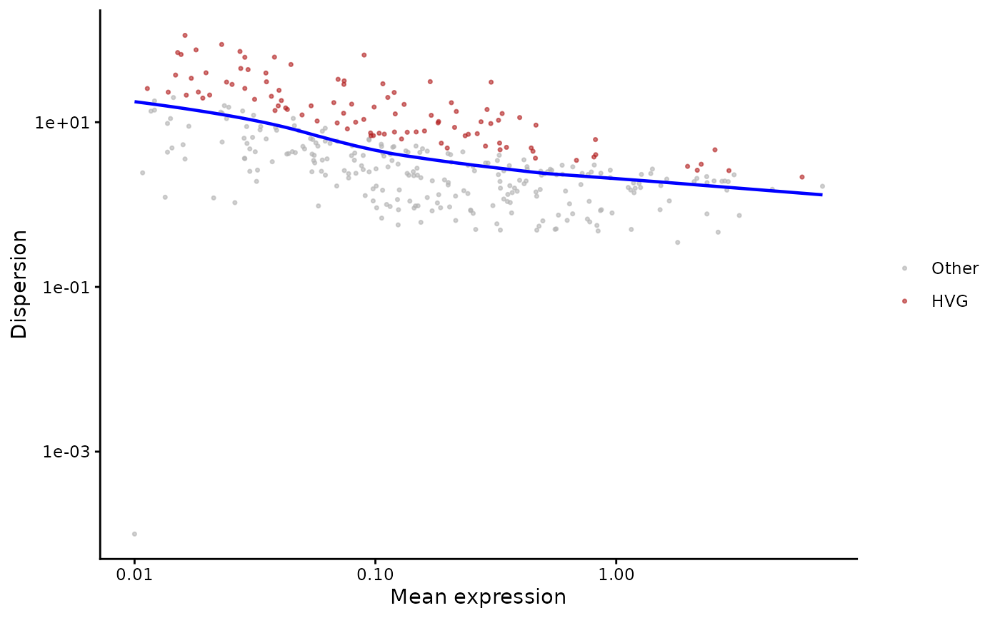
Visualises each eligible gene's dispersion against its mean expression,
overlaid with the fitted lowess trend, and highlights the selected highly
variable genes. Requires getHVG to have been run with a fitted
trend (i.e. more eligible genes than requested HVGs).
Usage
plotHVG(
  spe,
  pt.size = 0.6,
  pt.alpha = 0.6,
  cols = c("grey70", "firebrick"),
  line.col = "blue"
)
Arguments
- spe
A SpatialExperiment processed by
getHVG.- pt.size
Point size. Default 0.6.
- pt.alpha
Point alpha (0-1). Default 0.6.
- cols
Length-2 vector of colours for non-HVG and HVG points. Default
c("grey70", "firebrick").- line.col
Colour of the fitted trend line. Default "blue".